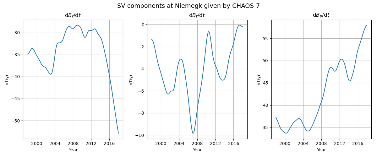
Evaluate CHAOS at a Ground Observatory

This script creates a time series plot of the first time-derivative of the magnetic field components (SV) by evaluating the CHAOS geomagnetic field model.

In this example the location of the ground observatory in Niemegk (Germany) is used. The spherical harmonic coefficients of the SV are truncated at degree 16. Note that the SV vector components are spherical geographic and not geodetic.

import chaosmagpy as cp
import matplotlib.pyplot as plt
import numpy as np

model = cp.CHAOS.from_mat('CHAOS-7.mat')  # load the mat-file of CHAOS-7

height = 0.  # geodetic height of the observatory in Niemegk (WGS84)
lat_gg = 52.07  # geodetic latitude of Niemegk in degrees
lon = 12.68  # longitude in degrees

radius, theta = cp.coordinate_utils.gg_to_geo(height, 90. - lat_gg)

data = {
    'Time': np.linspace(cp.mjd2000(1998, 1, 1), cp.mjd2000(2018, 1, 1), 500),  # time in mjd2000
    'Radius': radius,  # spherical geographic radius in kilometers
    'Theta': theta,  # spherical geographic colatitude in degrees
    'Phi': lon  # longitude in degrees
}

# compute SV components up to degree 16 (note deriv=1)
dBr, dBt, dBp = model.synth_values_tdep(
    data['Time'], data['Radius'], data['Theta'], data['Phi'], nmax=16, deriv=1)

fig, axes = plt.subplots(1, 3, figsize=(12, 5))
fig.subplots_adjust(
    top=0.874,
    bottom=0.117,
    left=0.061,
    right=0.985,
    hspace=0.2,
    wspace=0.242
)

fig.suptitle(f'SV components at Niemegk given by {model.name}', fontsize=14)

axes[0].plot(cp.timestamp(data['Time']), dBr)
axes[1].plot(cp.timestamp(data['Time']), dBt)
axes[2].plot(cp.timestamp(data['Time']), dBp)

axes[0].set_title('d$B_r$/d$t$')
axes[1].set_title('d$B_t$/d$t$')
axes[2].set_title('d$B_p$/d$t$')

for ax in axes:
    ax.grid()
    ax.set_xlabel('Year')
    ax.set_ylabel('nT/yr')

plt.show()