Usage
Here are some simple examples on how to use the package. This only requires a CHAOS model MAT-file, e.g. “CHAOS-6-x7.mat” in the current working directory. The model coefficients of the latest CHAOS model can be downloaded here.
Computing the field components on a grid
Use ChaosMagPy to compute the magnetic field components of the different sources that are accounted for in the model. For example, the time-dependent internal field:
import numpy as np
import chaosmagpy as cp

# create full grid
radius = 3485.  # km, core-mantle boundary
theta = np.linspace(0., 180., num=181)  # colatitude in degrees
phi = np.linspace(-180., 180., num=361)  # longitude in degrees

phi_grid, theta_grid = np.meshgrid(phi, theta)
radius_grid = radius*np.ones(phi_grid.shape)

time = cp.data_utils.mjd2000(2000, 1, 1)  # modified Julian date

# create a "model" instance by loading the CHAOS model from a mat-file
model = cp.load_CHAOS_matfile('CHAOS-6-x7.mat')

# compute field components on the grid using the method "synth_values_tdep"
B_radius, B_theta, B_phi = model.synth_values_tdep(time, radius_grid, theta_grid, phi_grid)
When using a regular grid, consider grid=True option for
speed. It will internally compute a grid in theta and phi similar to
numpy.meshgrid() in the example above while saving time with some of the
computations (note the usage of, for example, theta instead of
theta_grid):
B_radius, B_theta, B_phi = model.synth_values_tdep(time, radius, theta, phi, grid=True)
The same computation can be done with other sources described by the model:
Source |
Type |
Method in |
|---|---|---|
internal |
time-dependent |
|
static |
||
external |
time-dep. (GSM) |
|
time-dep. (SM) |
Computing timeseries of Gauss coefficients
ChaosMagPy can also be used to synthesize a timeseries of the spherical harmonic coefficients. For example, in the case of the time-dependent internal field:
import numpy as np
import chaosmagpy as cp

# load the CHAOS model from the mat-file
model = cp.load_CHAOS_matfile('CHAOS-6-x7.mat')

print('Model timespan is:', model.model_tdep.breaks[[0, -1]])

# create vector of time points in modified Julian date from 2000 to 2004
time = np.linspace(0., 4*365.25, 10)  # 10 equally-spaced time instances

# compute the Gauss coefficients of the MF, SV and SA of the internal field
coeffs_MF = model.synth_coeffs_tdep(time, nmax=13, deriv=0)  # shape: (10, 195)
coeffs_SV = model.synth_coeffs_tdep(time, nmax=14, deriv=1)  # shape: (10, 224)
coeffs_SA = model.synth_coeffs_tdep(time, nmax=9, deriv=2)  # shape: (10, 99)

# save time and coefficients to a txt-file: each column starts with the time
# point in decimal years followed by the Gauss coefficients in
# natural order, i.e. g(n,m): g(1,0), g(1, 1), h(1, 1), ...

dyear = cp.data_utils.mjd_to_dyear(time)  # convert mjd2000 to decimal year

np.savetxt('MF.txt', np.concatenate([dyear[None, :], coeffs_MF.T]), fmt='%10.5f', delimiter=' ')
np.savetxt('SV.txt', np.concatenate([dyear[None, :], coeffs_SV.T]), fmt='%10.5f', delimiter=' ')
np.savetxt('SA.txt', np.concatenate([dyear[None, :], coeffs_SA.T]), fmt='%10.5f', delimiter=' ')
The same can be done with other sources accounted for in CHAOS. However, except for the time-dependent internal field, there are no time derivatives available.
Source |
Type |
Method in |
|---|---|---|
internal |
time-dependent |
|
static |
||
external |
time-dep. (GSM) |
|
time-dep. (SM) |
Converting time formats in ChaosMagPy
The models in ChaosMagPy only accept modified Julian date. But sometimes it is easier to work in different units such as decimal years or Numpy’s datetime. For those cases, ChaosMagPy offers simple conversion functions. First, import ChaosMagPy and Numpy:
import chaosmagpy as cp
import numpy as np
From Modified Julian Dates
Convert to decimal years (account for leap years) with
chaosmagpy.data_utils.mjd_to_dyear():
>>> cp.data_utils.mjd_to_dyear(412.)
    2001.1260273972603
Convert to Numpy’s datetime object with
chaosmagpy.data_utils.timestamp():
>>> cp.data_utils.timestamp(412.)
    numpy.datetime64('2001-02-16T00:00:00.000000')
To Modified Julian Dates
Convert from decimal years (account for leap years) with
chaosmagpy.data_utils.dyear_to_mjd():
>>> cp.data_utils.dyear_to_mjd(2001.25)
    457.25
Convert from Numpy’s datetime object with
chaosmagpy.data_utils.mjd2000():
>>> cp.data_utils.mjd2000(np.datetime64('2001-02-01T12:00:00'))
    397.5
Note also that chaosmagpy.data_utils.mjd2000() (click to see
documentation) accepts a wide range of inputs. You can also give the date in
terms of integers for the year, month, and so on:
>>> cp.data_utils.mjd2000(2002, 1, 19, 15)  # 2002-01-19 15:00:00
    749.625
Plotting maps of the time-dependent internal field
Here, we make a map of the first time-derivative of the time-dependent internal part of the model. We will plot it on the surface at 3485 km (core-mantle boundary) from the center of Earth and on January 1, 2000:
import chaosmagpy as cp

model = cp.load_CHAOS_matfile('CHAOS-6-x7.mat')

radius = 3485.0  # km, here core-mantle boundary
time = 0.0  # mjd2000, here Jan 1, 2000 0:00 UTC

model.plot_maps_tdep(time, radius, nmax=16, deriv=1)  # plots the SV up to degree 16
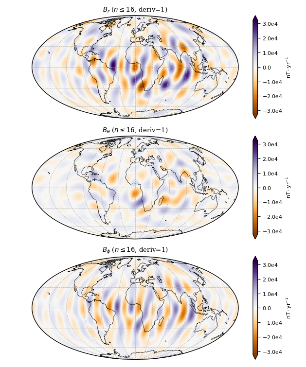
Secular variation at the core-mantle-boundary up to degree 16 in January 1, 2000 0:00 UTC.
Save Gauss coefficients of the time-dependent internal (i.e. large-scale core) field in shc-format to a file:
model.save_shcfile('CHAOS-6-x7_tdep.shc', model='tdep')
Plotting maps of the static internal field
Similarly, the static internal (i.e. small-scale crustal) part of the model can be plotted on a map:
import chaosmagpy as cp

model = cp.load_CHAOS_matfile('CHAOS-6-x7.mat')
model.plot_maps_static(radius=6371.2, nmax=85)
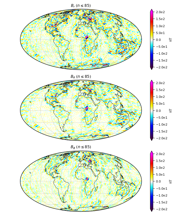
Static internal small-scale field at Earth’s surface up to degree 85.
and saved
model.save_shcfile('CHAOS-6-x7_static.shc', model='static')