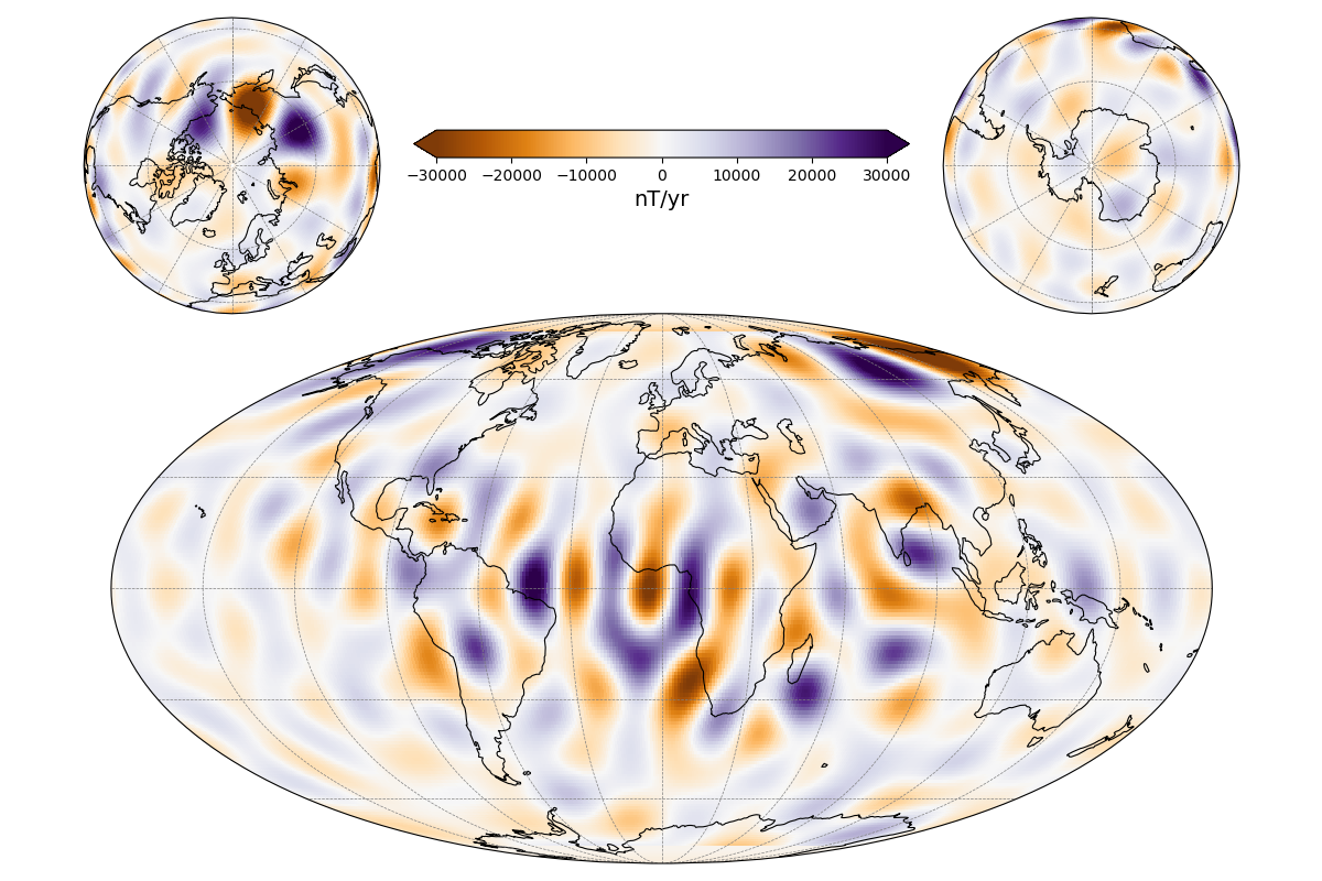
Create a Global Map and Polar Views

This script creates a map of the first time-derivative of the radial field component from the CHAOS geomagnetic field model on the core surface in 2016. The map projections are handled by the Cartopy package, which you need to install in addition to ChaosMagPy to execute the script.

# Copyright (C) 2024 Clemens Kloss
#
# This script is free software: you can redistribute it and/or modify it under
# the terms of the GNU Lesser General Public License as published by the Free
# Software Foundation, either version 3 of the License, or (at your option) any
# later version.
#
# This script is distributed in the hope that it will be useful, but WITHOUT
# ANY WARRANTY; without even the implied warranty of MERCHANTABILITY or FITNESS
# FOR A PARTICULAR PURPOSE. See the GNU Lesser General Public License for more
# details.
#
# You should have received a copy of the GNU Lesser General Public License
# along with this script. If not, see <https://www.gnu.org/licenses/>.

import chaosmagpy as cp
import numpy as np
import matplotlib.pyplot as plt
import matplotlib.gridspec as gridspec
from mpl_toolkits.axes_grid1.inset_locator import inset_axes
import cartopy.crs as ccrs

model = cp.CHAOS.from_mat('CHAOS-7.mat')  # load the mat-file of CHAOS-7

time = cp.data_utils.mjd2000(2016, 1, 1)  # convert date to mjd2000
radius = 3485.  # radius of the core surface in km
theta = np.linspace(1., 179., 181)  # colatitude in degrees
phi = np.linspace(-180., 180, 361)  # longitude in degrees

# compute radial SV up to degree 16 using CHAOS
B, _, _ = model.synth_values_tdep(time, radius, theta, phi,
                                  nmax=16, deriv=1, grid=True)

limit = 30e3  # nT/yr colorbar limit

# create figure
fig = plt.figure(figsize=(12, 8))

fig.subplots_adjust(
    top=0.98,
    bottom=0.02,
    left=0.013,
    right=0.988,
    hspace=0.0,
    wspace=1.0
)

# make array of axes
gs = gridspec.GridSpec(2, 2, width_ratios=[0.5, 0.5], height_ratios=[0.35, 0.65])

axes = [
    plt.subplot(gs[0, 0], projection=ccrs.NearsidePerspective(central_latitude=90.)),
    plt.subplot(gs[0, 1], projection=ccrs.NearsidePerspective(central_latitude=-90.)),
    plt.subplot(gs[1, :], projection=ccrs.Mollweide())
]

for ax in axes:
    pc = ax.pcolormesh(phi, 90. - theta, B, cmap='PuOr', vmin=-limit,
                       vmax=limit, transform=ccrs.PlateCarree())
    ax.gridlines(linewidth=0.5, linestyle='dashed', color='grey',
                 ylocs=np.linspace(-90, 90, num=7),  # parallels
                 xlocs=np.linspace(-180, 180, num=13))  # meridians
    ax.coastlines(linewidth=0.8, color='k')

# inset axes into global map and move upwards
cax = inset_axes(axes[-1], width="45%", height="5%", loc='upper center',
                 borderpad=-12)

# use last artist for the colorbar
clb = plt.colorbar(pc, cax=cax, extend='both', orientation='horizontal')
clb.set_label('nT/yr', fontsize=14)

plt.show()